Intercept Configuration

One of the most important configuration settings is the bounds on the intercept prior. The intercept prior controls the number of conversions (or amount of revenue) attributable strictly to organic conversions (absent marketing spend, promotional spikes, holidays, etc). We typically control this prior by setting three percentages: low-medium-high. These percentages are translated into strict prior bounds by doing the following:

• Calculate the median dependent variable for the previous 30 days before the as of date
• Multiplying the median by the lower and upper percentage
• A simulation is performed to ensure the mean of the prior distribution is approximately equal to the median dependent variable * the medium percentage

Note: Recast has more advanced methods for setting intercept priors, including priors that vary over time, but our default configuration uses a flat prior range over all timesteps.

Channel-Level Configuration

Upper Funnel vs Lower Funnel Channels

The first thing to decide about each marketing channel is whether it should be classified as an upper funnel channel or a lower funnel channel. Lower funnel channels are typically affiliate or paid search, where the amount paid is directly related to the sale event. When something is marked as a lower funnel channel, Recast will treat it special in a few ways:

1. Treat spend as an outcome, not just an input. This means that Recast will estimate a relationship between upper funnel spend and lower funnel spend. For example, we may estimate that for every $1k rise in TV, affiliate spend increases an extra $100 on average. We then use this information in forecasts, where the user only has to provide TV spend and we predict affiliate spend.
2. Reapportion credit to show a proper “total ROI” for upper funnel channels. The total ROI (shown on the Last Week Snapshot and whenever you select “Include lower funnel effects”) calculates the direct contribution of the channel, as well as the additional contribution from increasing spend in lower funnel channels, which then generate their own sales.
3. By default, lower funnel channels are excluded from time shift. Although override-able, this is the proper setting if the spend happens on the same day as conversion, such as when an affiliate program pays out whenever someone purchases.
4. By default, lower funnel channels are excluded from saturation. Although override-able, lower funnel channels are excluded from saturation by default because an increase in spend in something like affiliate (that may be juiced by upper funnel spend) should not see diminishing returns of incrementality.

ROI settings

ROI prior configuration

We specify a prior on the ROI by specifying a range that the ROI (or CPA) can be in at a particular price point. At higher price points the prior on the ROI will be lower, on lower price points the prior on the ROI will be higher. These ROI/CPA priors can be set arbitrarily, but we recommend a pattern for getting to a reasonable starting point for the priors. Internally we call it “napkin math.”

CPA Napkin Math

ROI Napkin Math

The logic of the napkin math works like this:

1. First, calculate the base CPA over a wide time period (all dollars spend divided by all conversions).
2. Then input the intercept percentage assumptions you made in the Intercept Configuration Section
3. By dividing the base CPA by 1-intercept percentage, we get the average CPA across all channels, if that was the true intercept percentage.
4. Then we spread these into a range by assuming that some channels at some points in time will be 3x worse than the average channel, while some channels at some points in time will be 3x better than the average.
   1. As one final edit, we recently started dramatically raising the upper bound CPA and setting the lower bound ROI prior to 0. We have found this better aligns with clients' incrementality tests (showing no lift at all) and their belief that some money is totally wasted.
5. We then take the range of these possibilities to get the range to use as our CPA prior.

We generally take the approach of applying the same ROI prior to all channels in the model. While true prior beliefs may vary about specific channels, we’ve found that in general tweaking priors to match customer expectations leads to a conflict where customers worry that we’re just engraining their own biases into the model. By using identical priors, we can be more confident that the posterior estimates are truly differentiated by data and not by different priors.

Exclude from saturation

We model the diminishing returns of a channel using the hill function (see our website for a introductory explainer). However, we also allow a channel to be excluded from saturating altogether, meaning that the estimated ROI will apply regardless of how much money is spent in the channel. This can be a useful assumption for lower funnel channels or channels where the diminishing returns are not expected until far greater levels of spend than are currently expected to be reached.

Saturation priors

We don’t typically specify priors on the parameters that control how fast the channel saturates. Instead we use the “Spend Level” to indicate a rough range for how big the channel can scale. We then do a simulation to find a prior on the saturation that allows for the possibility that the channel is very saturated at the “spend level” or very unsaturated at the “spend level.” If you find the model is expecting too much saturation, raising the “spend level” will lower the expected saturation and vice versa.

Non-Spend channels

In general, Recast usually recommends sticking to spend channels for predictor variables. However, our model can also incorporate non-spend predictors, like emails sent. These channels are not optimizable because they don't "compete" with other channels in the model for dollars; however, they can be used in forecasting. All other priors regarding predictor variables are still applicable, but special care should be taken in order to set reasonable ROI priors. While a 1x return on every dollar spent in Facebook may be reasonable, a $1 return for every email sent to a customer list is probably not.

Shift Settings

Shift prior configuration

For each channel, Recast estimates a shift curve to model the ad stock effect. This shift curve is constant across time, but different for each channel. The inputs to determine the shift curve are how many days it could reasonably take for 95% of the effect of spend to have been realized. We ask for a low-mid-high range of where this effect could be, and then back into the negative binomial parameters we use to parameterize the shift curve.

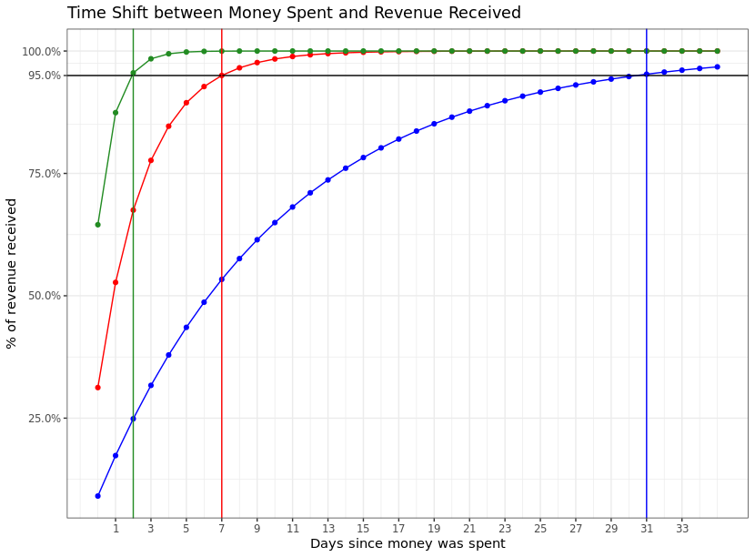
A low-mid-high range of 2, 7, and 31 means that our shift curve at it’s shortest could look like the green curve above (with over 60% of the effect happening on Day 0) and at it’s longest could look like the blue curve above (with about 10% of the effect happening on Day 0, and slowly petering out over time).

Exclude from shift

A channel can be excluded from shift, meaning that the full effect of the spend is realized on the day the money is spent.

Shift Concentration

The concentration parameter controls how right skewed the effect of spend is in the shift curve. If the concentration parameter is less than 1, the mode of the distribution (the day with the biggest effect) is Day 0. If the concentration parameter is greater than 1, the mode will be after Day 0.

For most channels, our opinion is that we should put strong prior weight on the channel having it’s mode close to Day 0. To this end, our default prior is a lower bound of 0.2 and an upper bound of 3.

Certain channels, however, can reasonably have a mode greater than 0. This can happen if there are two types of lag at play: a distribution lag and an adstock effect. For example, with direct mail, we typically record the spend on the day the mail goes to the post office. It will then take a few days for the mail to get distributed before the adstock effect takes effect. Podcasts can have a similar effect. For these channels we typically default to a concentration prior lower bound of 0.5 and upper bound of 10.

In the prior setting code, we support the following ConcentrationSetting options that set particular bounds on the Concentration parameter:

• 1 - this sets a lower bound of 0.2 and an upper bound of 1, for cases where there is no probability that the mode of the effect is greater than 0.
• 3 - this sets a lower bound of 0.2 and an upper bound of 3, our default prior for most channels
• 10 - this sets a lower bound of 0.5 and an upper bound of 10 (mean 3.5), our default prior for channels where we expect distribution lag (like mail and podcast)

Spike Configuration

Their are two types of spikes available in Recast:

• Additive spikes - these spikes model changes in the dependent variable directly. They’re called “additive” because they directly add to (or subtract from) the predicted dependent variable.
• Saturation Spikes - these spikes change the saturation multiplier, which multiplicatively effects the saturation point across all marketing channels. A saturation spike will make channels less saturated.

For convenience a spike can be marked as additive and saturation, although we treat these as two separate things within the model.

Additive spikes are typically used for promos and holidays where the dependent variable changes rapidly.

Saturation spikes are usually used around holidays, where the number of people in the market for a particular good rises quickly, thus making marketing more effective.

To configure a spike we need the following pieces of information:

• Spike group — each spike belongs to a group. The group is constructed using a Bayesian hierarchical model so that in the absence of data (like a spike in the future) the predicted performance will be similar to the in-sample spikes in the same group.
• Additive spike - Boolean - whether it’s an additive spike
• Saturation Spike - Boolean - whether it’s a saturation spike
• Main Date - The main date of the spike. Spikes can effect 30 days before and after the “Main date.” Their largest effect will be around the main date, while pull forward and pull backward effects of promotions will be included in the surrounding days. Typically we set the main date as the date in the promotional/holiday period with the highest sales.

Incrementality Tests

The Recast model incorporates lift test information by strongly constraining the prior during the time a lift test was run, thus ensuring the modeled results align with the lift test (within some margin of error), and adjusting the other ROIs in light of this information.

For general tips on how to actually translate client lift test data into an incrementality test for Recast, see this section.

The data Recast needs to implement an Incrementality Test is provided on the IncrementalityTests tab of the priors. In order to configure the test, we need the following pieces of information:

• Variable — Which marketing channel does the test apply to?
• Start date — When did the test start?
• End date — When did the test end?
• Point estimate — What was the mean estimate for the ROI (or CPA for CPA models)?
• Uncertainty — What standard error should we use? We use a N(point test, std err) to set the prior.
• Type — Should the prior apply to the ROI or the MROI?
  • For typical lift tests, the prior should apply to the channel’s ROI. Set the Type to “Average effect”.
  • If the lift test measured the effect of the just last dollar spent, rather than the total effect of the ad spend, then the prior should apply to the MROI. In this case (which is highly unusual) set the Type to “Incremental effect”.
• Time — How should the model take the test’s dates into account?
  • Setting Time to “Cumulative” applies the prior to the sum of the channel’s impact from the start date to the end date divided by the sum of the spend in the channel. This is the preferred option.
  • Setting Time to “Daily” applies the prior separately to every day’s ROI from the start date to the end date. Due to variations in spend from day to day, it is likely that each day has a slightly different ROI, so this may not be a realistic assumption.
  • Setting Time to “Bookend” applies the prior separately just to the ROIs on the Start date and End date.
• Include lower funnel effects — Not supported currently (for future use)

Contextual Variable Configuration

Contextual variables are variables that indirectly effect the dependent variable by changing the organic effectiveness and the effectiveness of marketing. A classic example is when a company raises prices. The number of conversions will likely fall, and this fall will be attributable to a drop in the number of organic conversions, as well as less efficient marketing spend (as customers are turned off by the price point). Instead of attributing conversions to this variable directly, we model a multiplicative effect on the intercept/spikes and ROIs. We can shorthand the equations as:

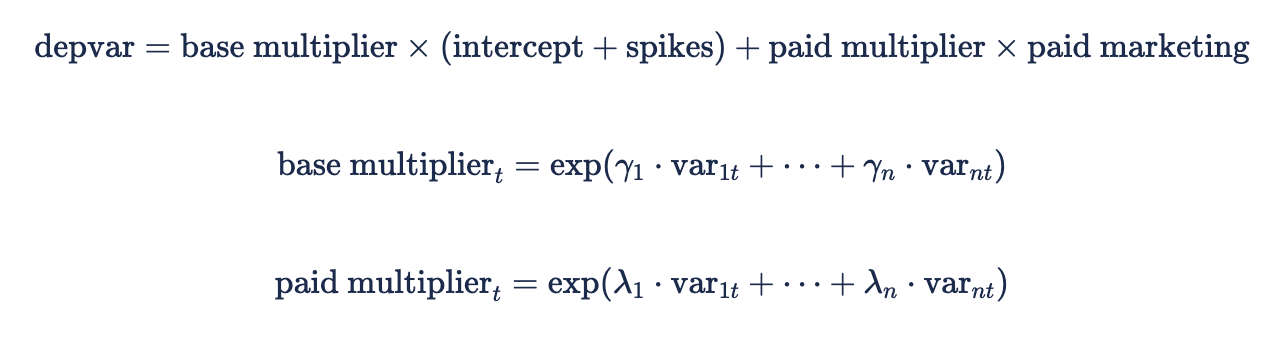
The above equation says that the base multiplier at time t is the exponentiated sum of each contextual variable at time t multiplied with the estimated contextual variable effect gamma.

This model assumes that the context variable has the same multiplicative effect on all channels ROIs.

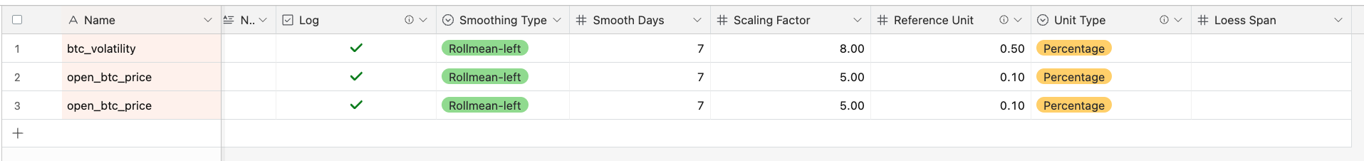
In order to configure a contextual variable, you supply it as a column in clean_data and then specify it on the ContextVariables tab during prior setting. The app automatically supports three common types of transformations you might want to do on the contextual variables. This means that you can supply the variables without applying the transformations, and when someone uses the app to run forecasts/optimizations they can supply the variable in the natural units they’re used to that will then be automatically translated to the modeled units behind the scene.

The three transformations are:

1. Logging - take the natural log of the contextual variable (see below for how this changes the interpretation).
2. Smooth - applies a smoothing operation to the dependent variable (ensuring the day to day variation isn’t too jumpy), two types:
   1. Rollingmean - take a rolling mean, the alignment (center, left, or right) and the window size are configurable
   2. Loess smoothing - the span parameter is configurable
3. Scaling - Dividing by a constant in order to make the range appropriate for the prior (which does not change)

Interpretations

When logging, the interpretation is: an x% change in the context variable has a y% change on the marketing (or organic) effectiveness

When not logging, the interpretation is: an x unit change in the context variable has a y% change on the marketing (or organic) effectiveness

The smoothing operation does not change the basic interpretation, although it will change how reactive the model is to the change in contextual variable.

Scaling

Scaling the context variable is important because we use a constant prior N(0, 1) on all the effects.

A baseline recommendation (which can be customized for specific cases) is to scale the data such that there is roughly a 0.5 range from the min to the max of the data. If we take 3 as a large, but not impossible posterior mean from a standard normal prior, this means at the two extremes of the data we will have:

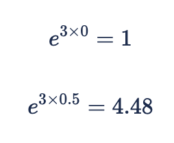
In other words, marketing (or organic) effectiveness will be 4.48x higher at the peak of the context variable than at the lowest point. The larger the range of the data, the bigger the prior difference in multipliers from the top of the scale to the bottom.

Note: in order to figure out the proper scale, you must take the log first if you are logging. While it may seem it would be convenient to set the ending range you want in directly in the prior inputs (for example, use whatever scaling factor gives a 0.5 range), this is not ideal because it is equivalent to calculating the prior from the data, which will lead to changing priors every time the range of the observed data changes.

There are two additional parameters that are configurable in the Google Sheet/Airtable, which do not change the model, but customize how we display the results in the dashboard.

Unit Type defines how we customize the units in the interpretation text provided in the contextual variable summary. There are five options currently:

1. Percentage - the only acceptable option if logging the depvar (an error will throw if Percentage is not used when logging). When using Percentage, the Reference Unit refers to the percentage increase you want to use to demonstrate the effect. If it’s 0.1, the interpretative sentence will be “For every 10% increase in context var, the marketing effectiveness will change by ….”
2. Units - When the context variable refers strictly to a count of something
3. Currency - when the context variable refers to a monetary amount. The text will be formatted with the proper currency symbols.
4. PercentagePoint - when the context variable refers to a percentage, as in brand awareness surveys. This assumes the raw variable is in the interval [0-1]
5. Binary - when the context variable refers to an on or off state, like a one time price increase.

Reference Unit allows you to customize the sentence because the traditional statistical interpretation (”a one unit increase in x leads to a …”) may not be helpful if the units are measured in millions or hundredths. It should be selected to be whatever a normal, meaningful change in the context variable would be to the client (on the client’s scale, not the transformed scale). When Unit Type is binary, it should always be 1.

Context Variables and Budgets

Currently goals, optimizations, and forecasts can handle context variables in two ways:

1. User does not provide — in this case, the last value in the in-sample data is carried forward for the out of sample data. In many cases this might be our “best guess” of what the future holds.
2. Clients provide the data in the format they originally provided the data. The three transformations will happen automatically by the app.