
Introduction
Under the hood, Recast fits a statistical model to your data. The model is a Bayesian hierarchical time series model and the fitting happens via a Hamiltonian Monte Carlo (HMC) algorithm in Stan.
The documentation below covers the core parts of the statistical model as they are specified mathematically. Since there’s a lot of very dense information here, we’ll start by laying out the model's assumptions in prose before getting into the formal specification.
To start, let’s lay out a diagram of how we believe marketing performance actually works. This causal diagram is designed to help us think from first principles about 1) what are the true causal relationships we are trying to understand and 2) how we can build a statistical model that estimates the relationships of interest.
The causal diagram looks like this:
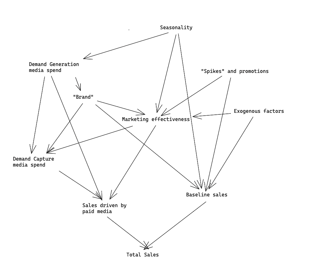
It’s complicated! Marketing is a complicated domain and there are lots of factors that impact each other in non-obvious and non-measurable ways. Our job as modelers is to build a statistical model that can estimate the most important relationships in this causal diagram in a way that’s robust and unbiased.
The Recast statistical model is a fully Bayesian generative model that attempts to capture all of these relationships in code. The core model includes thousands of lines of Stan code which we won’t walk through, and instead, we’ll outline the core components and how the pieces fit together.
Core assumptions:
-
The dependent variable is impacted by
-
Paid media performance.
-
Baseline non-media sales or the “intercept”.
-
“Spikes”: exogenous shocks, usually from holidays, promotions, or new product launches.
-
“Contextual variables” which have their impacts through the intercept and paid media variables.
-
-
Paid media performance has the following characteristics
-
Marketing performance can change over time, but the changes must be smooth according to a Gaussian process
-
The effect of marketing is shifted in time according to a negative binomial distribution
-
There are diminishing marginal returns to increased investment in Paid media. I.e., marketing channels “get saturated”
-
Marketing performance may be impacted by seasonal trends (i.e., channels might get more performance in the summer vs. the winter).
-
-
The intercept has the following characteristics
-
The intercept changes over time, but the changes must be smooth according to a Gaussian process
-
The intercept may be impacted by seasonal trends (i.e., it may be higher in the summer vs. the winter).
-
-
Spikes have the following characteristics
-
Spikes may have pull-forward and pull-backward effects (i.e., they distort sales that were going to happen before or after the spike date)
-
Spikes may interact with marketing performance (you can spend more money in certain marketing channels when a promotion is happening)
-
Now, let’s get into the math!
Preliminaries
Time-varying coefficients
Several things change over time in Recast’s model:
-
The intercept
-
The ROIs of media channels
-
Crucially, as we’ll explain below, this contains two time-varying components for each channel. One is the performance of the “first dollar” of spend in the channel (and — if not indexed by spend, the equivalent “first activity”), and the other is a shared “saturation multiplier” — this will make more sense below.
-
-
The saturation multiplier
All of the parameters that change over time are assumed to follow a locally-periodic Gaussian Process. You can read more about locally periodic kernels here, but the gist is that the kernel makes three assumptions:
-
Today is like yesterday
-
Today is like one year ago
-
Today is more like one year ago than like two years ago
For details on our implementation of locally-periodic Gaussian processes, see our doc Mean-Zero Gaussian Processes: An Overview.
The Intercept
The functional form of the intercept is the following:
Where:
-
lb and ub represent the upper and lower bounds for the intercept
-
mean and trend represent the latent linear trend in the intercept
-
GP is a locally-periodic Gaussian Process
ROIs — direct and indirect
Direct effects
The effect — before time-shifting (see below for how we estimate the time-shifting) — of marketing activity in a channel c at time t is given by the following formula:
We have a section on the Hill Function below — this is how we model the “saturation” effect. The kappa term in there can be thought of as the amount that one can spend into that channel before the channel gets saturated. The beta term can be thought of as the efficiency of this saturated spend.
In turn, the kappa term is itself the product of two components:
We model a saturation term for each channel, and a multiplier term for each time step. This multiplier term is the same mentioned above – it evolves according to a locally periodic Gaussian Process, which allows for the overall saturation level across a model to go up and down with the seasons and over time.
The beta term is itself indexed by channel and time step — we model it with a locally periodic GP for each channel.
The time-varying multiplier
The specification for the time-varying multiplier is as follows:

where:
-
lb and ub represent the upper and lower bounds for the multiplier
-
mean and trend represent the latent linear trend in the multiplier
-
GP is a locally-periodic Gaussian Process
-

Indirect effects and the difference between “demand generation” and “demand capture” channels
Recast has two different types of channels — those whose spend levels can be directly manipulated by the advertiser, and those – like branded search or affiliate — whose spend levels are essentially “taken” by the advertiser. We call these “demand generation” and “demand capture” channels, respectively.
In order to capture this dependence in induced spend in demand capture channels that is driven by activity in demand capture channels, we include the following in our model:

That is, the amount of spend in the lth demand capture channel at the tth time step is a function of:
-
Some baseline level of spend (the intercept term) — that evolves according to a GP
-
The shifted effects of each demand generation channel multiplied by an alpha coefficient for each pair of demand generation and demand capture channels
Therefore the total effect of a demand generation channel will be:
-
The direct effect of spend into the channel
-
Plus the effect of the induced spend into the demand capture channels that it influenced
-
Which will depend both on how strongly the demand generation channel influences that capture channel, and
-
How effective the capture channel is
-
Importantly — both demand generation and capture channels have direct effects!
The model’s basic formula
The dependent variable or depvar is modeled in terms of a time series model, with the basic formula given as:
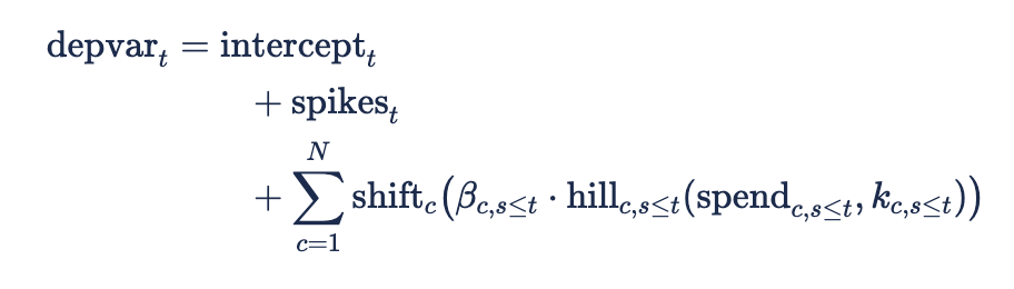
Where:
-
t indicates time step and c indicates channel
-
N is the number of channels.
-
Importantly, N is inclusive of demand generation and demand capture channels — in the prediction of the outcome variable (e.g. revenue or conversions), they have the same functional form
-
-

-

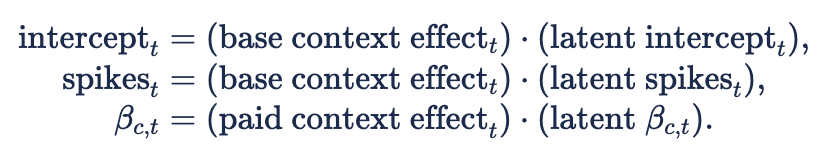
-

In this formula, the betas, intercept, and spikes may also include exogenous contextual effects:
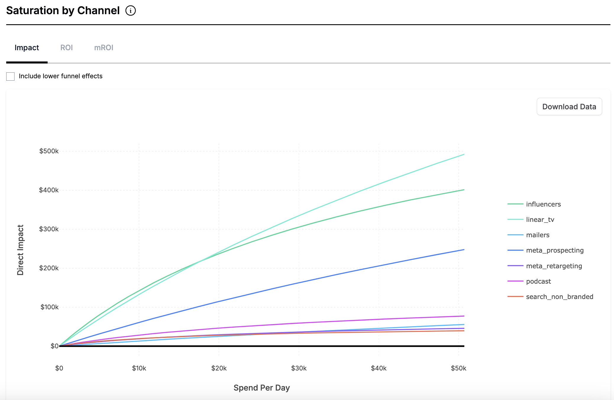
Hill saturation function
We assume that channels saturate — meaning that as you spend more and more you get less and less return. This plot shows how the ROI is expected to change at different levels of daily marketing spend for each channel:
We do this by using a single parameter Hill function, also called the Monod equation.
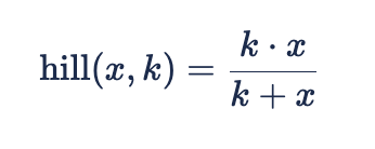
Here, k is the saturation point - you can never get more “effective dollars” out of the channel than the saturation point. We estimate a saturation point for each channel - ![]()
Our model precludes the possibility of an “activation” effect.
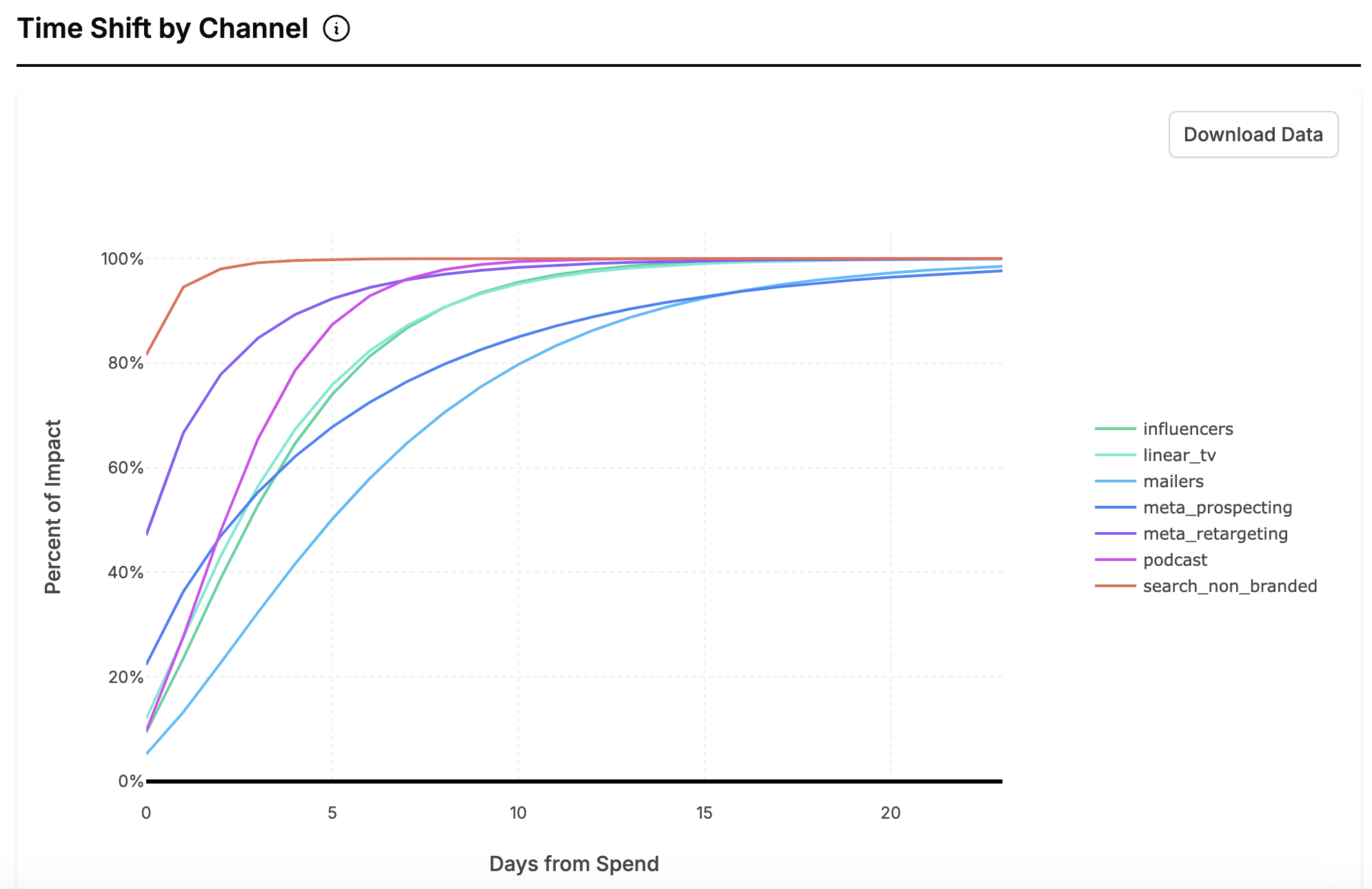
Time Shifts
The effect described in this equation is in a sense “all of the effect that will ever happen” because of spend on a given day. E.g. if the estimated ROI is 2x and spend is $100, this would mean that the unshifted effect would be $200. But Recast would not predict that revenue would go up by $200 on that day — the $200 would be distributed over time; perhaps $100 on the day of spend, $50 on the day after that, $30 on the third day, and $20 on the fourth.
In order to shift the effect over time, we use the negative binomial distribution. It is convenient as it is a probability mass function with support on the non-negative integers — so we know that the weights will add up to one, and the values you can plug into it map nicely to the idea of “days after spend”. It also takes the shapes that we believe make sense for how effects should be distributed over time — ranging from very quick decays to slow builds.
Spikes & Spike Groups
We model promotional activity and holidays through “spikes”. Unlike a dummy variable, we assume spikes may have pull-forward and pull-backward effects (i.e., they distort sales that were going to happen before or after the spike date) and that spikes may interact with marketing performance (you can spend more money on certain marketing channels when a promotion is happening).
Here’s how spikes could look in practice:
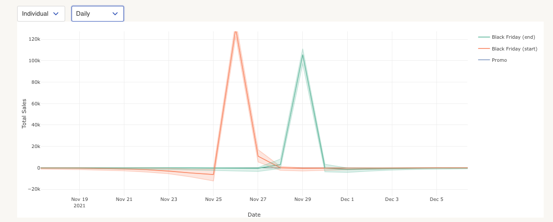
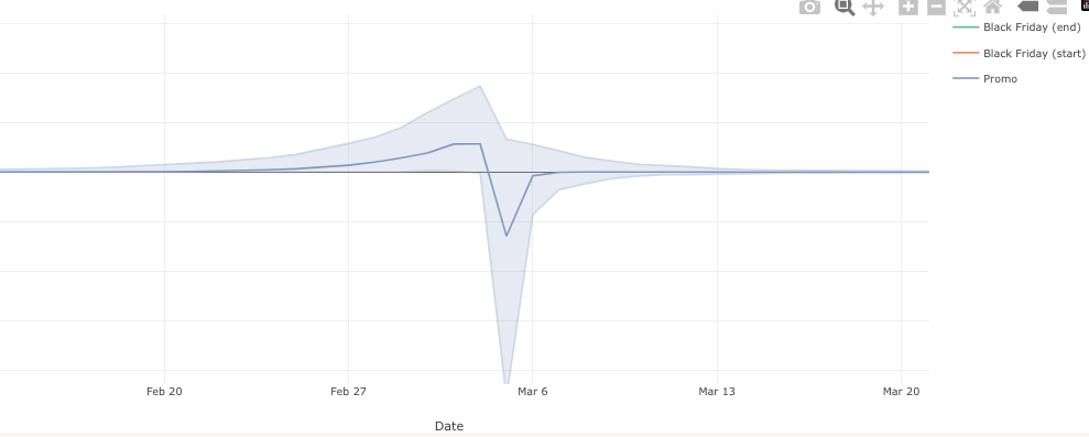
The important features of the spikes is that they can be negative — before, after, or during the promotion. But they are not guaranteed to be — they can be purely positive as well.
The overall effect of spikes can also be negative, positive, or close to zero.
Spike parameterization
We achieve this flexibility with a simple parameterization: we use a mixture of two asymmetric double exponential variables:
where Y_1 and Y_2 are densities of the Asymmetric Laplace distribution, defined by

-
The first of the three parameters, m, controls overall magnitude (bigger number, bigger magnitude).
-
The second parameter,

-
The third parameter,

All parameters are strictly positive.
The following code in R computes the density of an asymmetric Laplace:
spike_kernel_val = function(x, center, mag, skew, spread){
   y =  spread * (x - center)
   z = spread / (skew + 1/skew)

   second_term = ifelse(test = x < center,
                         yes = exp(y/skew),
                          no = exp(-y*skew)
                        )
   return(mag*z*second_term)
}
Spike Groups
Most “spikes” are things like “Christmas” or a “Mother’s Day Sale” or things like a “20% off Sale”. That is to say, there should be some notion of grouping — when Christmas is coming, we should be able to forecast the effect of Christmas based on past Christmases, and when the model has seen the data, other Christmases should inform its estimate of the effect of the holiday.
In order to capture this notion of grouping, we have spike groups. For each spike group (one group could represent “Christmas”, but not a specific Christmas), we estimate the six parameters discussed above. But for each spike (e.g., 12/26/2022 — that is, a specific Christmas), we estimate six more parameters, each corresponding to one of the six:
This induces a distribution centered around 1 — more tightly distributed around 1 as similarity increases. Then the parameters we plug into the Asymmetric Laplace distributions above are simply:
Linking parameters within and across models
In general, the interpretable parameters that come out of Recast have the following quality: they are a set of transformations applied to a latent parameter, which is typically standard normal. For example, the transformations applied to get the shift curve are:
-
The latent parameters are two variables with a standard normal prior
-
Each latent parameter is pushed through a shifted and scaled inverse logit transformation
-
These two transformed parameters are then used as the mean and concentration of a negative binomial distribution
The transformation to obtain the betas is the following:
-
A time series of variables with a standard normal prior are sampled
-
They are multiplied by a locally-periodic kernel to obtain a Gaussian Process
-
This GP is then pushed through a shifted and scaled inverse logit transformation
In Recast, the linking happens at the latent parameter level. The linking happens in the following way. Say that we have a set of linked models representing New York and California, and that we have local TV spend in both markets. We want our links to represent both information-sharing between all channels in New York, and one representing information-sharing between both TV channels.
The result for “TV in New York” would then be the following:
tv_ny = weight_ind * ind_contrib + weight_ny * mean_ny + weight_tv * mean_tv
Where
-
tv_nyrepresents the latent parameter of interest -
ind_contribrepresents the “individual contribution” or deviation from the group means -
mean_nyrepresents the overall mean for New York channels -
mean_tvrepresents the overall mean for TV channels -
weight_*represents the contribution of each parameter to the final result. These weights sum to 1
The weight_* parameters are calculated in the following way. For each linking level (here there are two, but in general there can be any number), we sample a parameter representing the strength of that linking. The prior on this parameter contains information about our expectation of the strength of the linking as well as our confidence in that value.
The process works in the following way:
for(i in 1:n_groups) {
	latent_weights[i] ~ normal(strength_of_grouping[i], confidence_in_grouping[i])
}

weights = softmax(latent_weights)
This setup is nonstandard but it allows us to have several capabilities:
-
We can have a variable number of links for any channel (in this case, both channels in the New York market and channels that represent TV spend are linked together)
-
Because we do the information-sharing at the latent-parameter level, it allows us to link together parameters that may end up at different scales after we apply the transformations specific to that parameter. For example, we may link together the betas for a CPA based model (where we would expect the beta to be on the order of 1/100, representing a $100 CPA) and an ROI based model (where would expect the beta to be on the order of 2). If TV is “better than expected” in one model, that provides information that it should be better than expected in another model
-
Our priors can inform the expected strength of linking, and the model can confirm or override our priors. If the
latent_weightsend up as strongly negative, theweightswill approach zero, leaving only the “individual contribution”, meaning the results will be as if there was no linking whatsoever