
This document explains how Recast incorporates incrementality tests into its MMM. If you haven’t yet, read our experiments documentation for an overview of how we think about and analyze incrementality tests.
Holdout (Average Effect) Tests
In a holdout test, the tested channels are turned off entirely in one test cell and are kept as business as usual in the other test cell. The difference in outcomes between the two test cells gives you the channels' total effect, and dividing by the channels' spend during the test gives you an ROI. The model constrains its own estimate of the channels' ROI to be consistent with this measured ROI.
What the model computes
For each day during the test, the model has an estimate of each channel's effect -- the contribution of that channel's spend to the KPI (e.g. revenue) after accounting for saturation. The model also knows each channel's spend.
For all channels in the test, the model sums up the effects and the spends over the test period, then divides to get a modeled ROI:
By default, effects and spends are summed over the full test period when computing this ROI.
Note that the model uses the unshifted effect here (the effect before applying the channels' time shifts). The actual test outcome inherently includes the delayed effects of spend during the test period, and the unshifted effect is a reasonable approximation of that as long as the test runs long enough or the test's analysis includes a sufficient cooldown period after the test ends.
Including lower funnel effects
When we instruct the model to include lower funnel effects, the total effect of the tested channels also includes an approximation of the indirect impact that the tested upper funnel channels have on lower funnel channels. For example, if TV spend drives paid search activity, the revenue attributable to that driven search activity is part of what the real-world test measured.
To avoid double counting, this indirect effect only flows through lower funnel channels that are not themselves part of the test. If a lower funnel channel is being directly tested, its effect is already in the numerator from the direct effect sum.
The full ROI with lower funnel effects is:
The prior
The modeled ROI is compared to the point estimate and uncertainty from the test:
The available distributions are Gaussian, Strict Gaussian, and Uniform.
Multichannel holdout tests
A holdout test can involve multiple channels -- for example, turning off both Linear TV and OTT in the treatment cell. In that case, the numerator sums effects across all tested channels (both upper and lower funnel), and the denominator sums their spends. The resulting ROI reflects the combined efficiency of all channels in the test.
Impact Tests
Why impact tests need special handling
Impact tests are different from holdout tests. Both cells have spend, possibly at different levels. The difference in outcomes between the cells reflects only the effect of the difference in spend -- a slice of the channels' saturation curves, not the whole thing. Converting that to an ROI would produce a number that isn't comparable to the model's overall ROI. So instead of constraining the model's ROI, we constrain the model's predicted difference in impact between the two cells.
Definitions
We'll call the cells of the test "cell 1" and "cell 2". For an impact test, we need four cell parameters:
-
Typical spend proportion for each cell (
p_1andp_2): what fraction of the tested channels' total spend typically occurs in each cell's geographic region. For example, if cell 1 covers a region that normally accounts for 25% of total spend, thenp_1 = 0.25. -
Test spend ratio for each cell (
r_1andr_2): how much spend in the tested channels was scaled relative to typical levels during the test. For example, if spend in cell 1 was doubled,r_1 = 2. If spend was held at its usual level,r = 1. If spend was turned off,r = 0. These ratios apply to all channels in the test.
Estimating spend in each cell
The model observes only each channel's total daily spend across the entire market, not spend at the cell level. We estimate cell-level spend by scaling the observed total using the cell parameters.
For each channel in the test, we take its total daily spend and scale it according to each cell's typical size and how much spending was changed relative to baseline. We also need to adjust for the fact that the test may have changed total observed spend. For instance, if both cells scaled spend up, the observed total is higher than it would have been otherwise. The adjustment factor is:
The estimated daily spend in each cell is then:
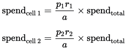
Of course, actual cell-level spend will differ somewhat from this formula -- real spend patterns are more complex than a proportional split. But this approximation captures the right magnitude and day-to-day variation, which is what matters for the saturation calculations described next.
Why saturation matters
The MMM models diminishing returns. Doubling a channel's spend doesn't double its effect; at higher spend levels, each additional dollar buys less.
Impact tests need to account for this because each cell may sit at a very different point on the saturation curve. One cell might be spending at 2x normal (deep into diminishing returns) while the other is at 0.5x (where spend is more productive). In contrast, a holdout test's "treatment" cell runs at roughly market-level saturation, so the model's standard parameters apply directly.
To account for this we apply the saturation function separately to each cell's estimated spend, using a saturation parameter scaled to the cell's size:
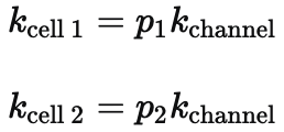
k_channel is the model's saturation parameter for a given channel in the full market. Scaling by p reflects the fact that a cell representing 25% of the market saturates at roughly 25% of the level the full market would. We do this separately for each channel in the test.
Computing the effect difference
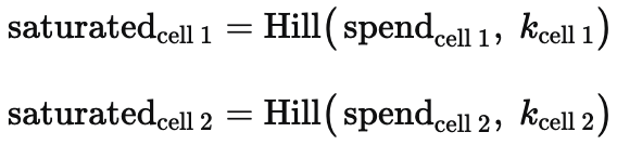
For each day during the test and each channel in the test, the model:
-
Applies the saturation function to each cell's estimated spend with the cell-specific saturation parameter:
-
Multiplies by the channel's effectiveness parameter
betaand takes the difference:
When the test involves multiple channels, these per-channel effect differences are summed.
Including lower funnel effects
When "include lower funnel effects" is enabled, the model also captures the indirect impact that upper funnel channels have on lower funnel channels. If an upper funnel channel like TV drives more awareness in cell 1 than cell 2, that difference ripples through to lower funnel channels like paid search, creating an additional difference in outcomes between the cells.
The model approximates this indirect effect and adds it to the effect difference. To avoid double counting, it only includes indirect effects flowing through lower funnel channels that are not themselves part of the test. Any lower funnel channel that is directly manipulated in the test already has its direct effect counted in the main calculation above.
Accounting for unequal cell sizes
When the two cells represent different fractions of the market (p_1 != p_2), non-test contributions to outcomes don't cancel in the subtraction. Baseline demand and effects from channels not in the test will all be proportionally larger in the bigger cell.
The model corrects for this by estimating these non-test contributions and scaling by the cell size difference:
This way, the predicted cell difference reflects the effect of the tested channels plus the expected baseline difference from the size mismatch.
The prior
The model's total predicted difference between the two cells is:
We compare this to the point estimate and uncertainty from the test:
The available distributions are Gaussian, Strict Gaussian, and Uniform, the same as for other test types.
Both the test effect and other effect terms are summed across all days in the test before the comparison, so the prior is applied cumulatively. The point estimate should represent the total difference in outcomes (e.g. total incremental sales) over the entire test period.
Saturation correction during the test period
During the test, the redistribution of spend across cells slightly changes each tested channel's overall saturation in the market, even if total spend stays the same. Consider two cells each representing a third of the market: cell 1 cuts spend by half while cell 2 increases it by 50%. Total spend is unchanged, but because the saturation curve is concave, the combined effect of spend distributed this way differs from the effect of the same total split evenly across the cells.
The model adjusts its saturation parameters for each tested channel during the test period to account for this, preventing the test's spend redistribution from biasing estimates of channel effectiveness outside the test cells.
Multichannel impact tests
Impact tests can involve multiple channels simultaneously -- for example, scaling both Linear TV and OTT in one cell while keeping them business as usual in the other. When a test involves multiple channels:
-
The effect difference is computed separately for each channel and then summed before the prior is applied.
-
If lower funnel effects are included, indirect effects from all upper funnel channels in the test are counted, but only through lower funnel channels not themselves in the test.
-
The cell parameters (typical spend proportions and test spend ratios) apply uniformly to all channels in the test, meaning the test design assumes all tested channels were scaled by the same factor in each cell.