Mean-Zero Gaussian Processes: An Overview

One available option for the MMM’s time-varying parameters are our so-called mean-zero Gaussian processes.

Straight to the definition

We’ll explain the definition of a mean-zero Gaussian process (GP) by contrasting it with a typical GP.

Typical Gaussian processes

A typical (non-mean-zero) GP can be defined as

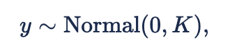
where ‘y' is a parameter vector with one entry for each time step and 'K’ is a covariance matrix built from the GP’s kernel function.^[1] We’ve used a prior mean of zero here for simplicity.

Instead of sampling from that multivariate normal directly, we can first calculate the Cholesky decomposition K=LL^T , where L is a lower triangular matrix with positive diagonal entries and L^T is its transpose. Multiplying that matrix L against a vector of parameters sampled from independent standard normal distributions is equivalent to sampling from the above multivariate normal. In other words, we have this alternative implementation of the typical GP:

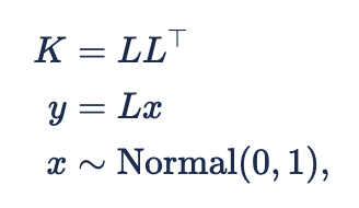
where x now the parameter vector. This is equivalent to the definition above.

Note that, even though the expected prior mean of 'y' is zero, its posterior mean (after fitting it to data) is not necessarily zero.

Mean-zero Gaussian processes

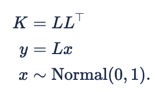
We define a mean-zero GP starting from the Cholesky decomposition implementation

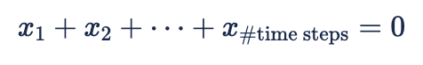
First we place a sum-to-zero constraint on 'x':

We then define

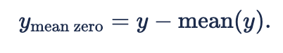
This is the mean-zero GP.

Applications in the MMM

We use these mean-zero GPs to build the MMM’s time-varying parameters.

Suppose we want to build a channel’s beta parameter,

First we build a vector on unconstrained space by mixing the mean-zero GP with a scalar parameter 'w' :

where

• is a scalar between 0 and 1,

• is a scalar with

• and is a mean-zero GP. We scale it so that each entry of has a prior variance of 1.

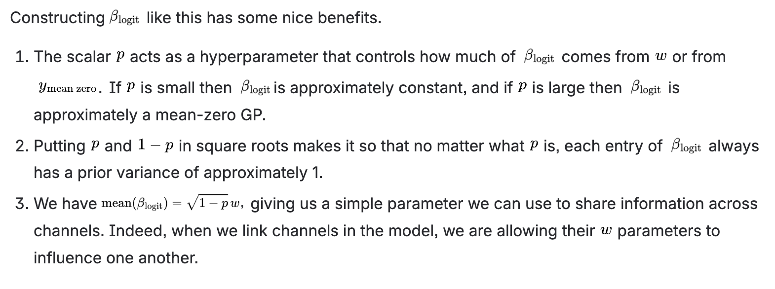
We construct the final beta parameter using the inverse logit transform:

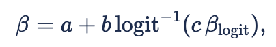
where are constants we can use to set appropriate priors on

We use this construction for essentially every time-varying parameter in the MMM.

Why?

Appendix: Motivation for the construction

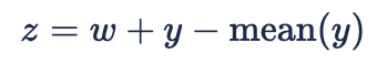
The original motivation for mean-zero GPs came from wanting a single parameter 'w' that acted as the mean value of the GP.

Naively we tried taking a typical GP ‘y' and a scalar 'w' and defining a time-varying parameter 'z’ like

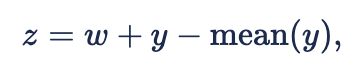
but ran into a major issue. It turns out that when you use the Cholesky decomposition method to build the 'y' for this, 'x' becomes nonidentifiable.

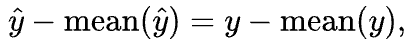
If then define alternate versions of ‘x' and 'y’ -- we’ll call them -- by

where 'c' is any scalar. Then

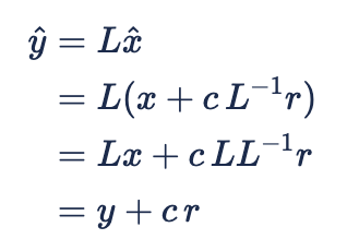
and so

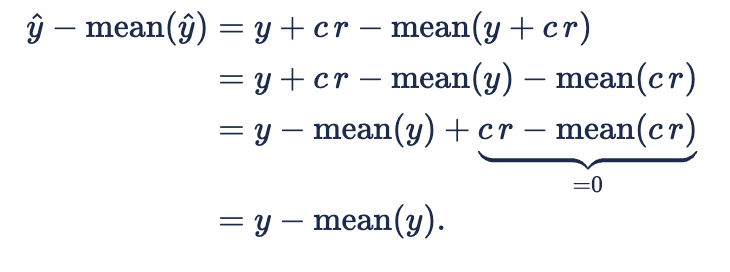
Since we’ve found infinitely many different values of ‘x' (since ‘c’ was arbitrary) that produce the same 'z’.

You might be interested to see what that vector looks like. Here’s a plot using one of our usual kernels:

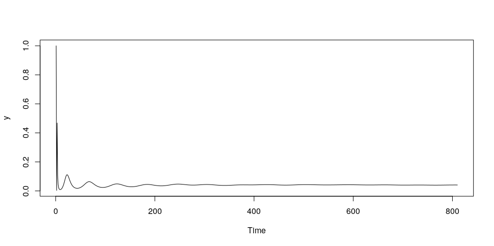
What can we do to constrain ‘x' so that it can’t move along this problem vector? Well, since this problem vector changes the sum of ‘x’, we could try restricting 'x' so that its sum is zero.

If we force ‘x' to sum to zero, we effectively restrict our GP ‘y’ to a subset of all typical GPs. How much does this constrain 'y’ ? Not much, it turns out. We can easily generate some data to try fitting it with these constrained GPs, and in doing so we found that the constrained GPs behave quite similarly to unconstrained GPs.

The final step, going from

to

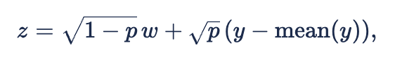
gives us a new hyperparameter ‘p' that controls how constant-like ‘z’ is. We could achieve a similar result by changing the variance hyperparameter in the GP kernel, but by doing it this way we don’t need to worry about balancing the prior variances of ‘y’ and 'w’.

Footnotes

[1] A great intro to Gaussian processes is Yuge Shi’s “Gaussian Processes, not quite for dummies”, The Gradient, 2019.