⏏️ Interpreting the Outputs

Recast will produce a variety of outputs available to Partner data scientists. This page summarizes how to interpret the important information in these outputs.

The Run Analysis Dashboard

The primary purpose of the run analysis dashboard is to compare two runs that differ either in the data used or the model configuration. It allows us to see how things are different in terms of input data, priors, and results. Run analyses are created in the following situations:

When a normal run is finished, it will create a run analysis dashboard comparing the latest run with whatever run has been 'activated' most recently. If there are no activated dashboards, the run analysis won't be created.
When a stability loop is run, each model run is compared to the previous time period's model run.
[COMING SOON] A tool to dynamically create these dashboards between any two runs. If this is a blocker for you, please reach out to Recast for assistance.

As this has primarily been an internal tool, the graphs can be a bit complex and opaque, but I will touch on the major things worth paying the most attention to below.

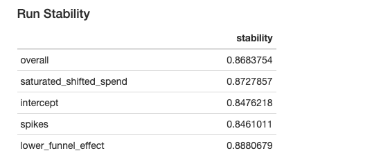
The Run Stability metrics provide a percentage overlap in the key model components between the old run and the new run. A score of 1 would mean the model was exactly the same as the previous. Values over 0.8 are typically considered "stable."

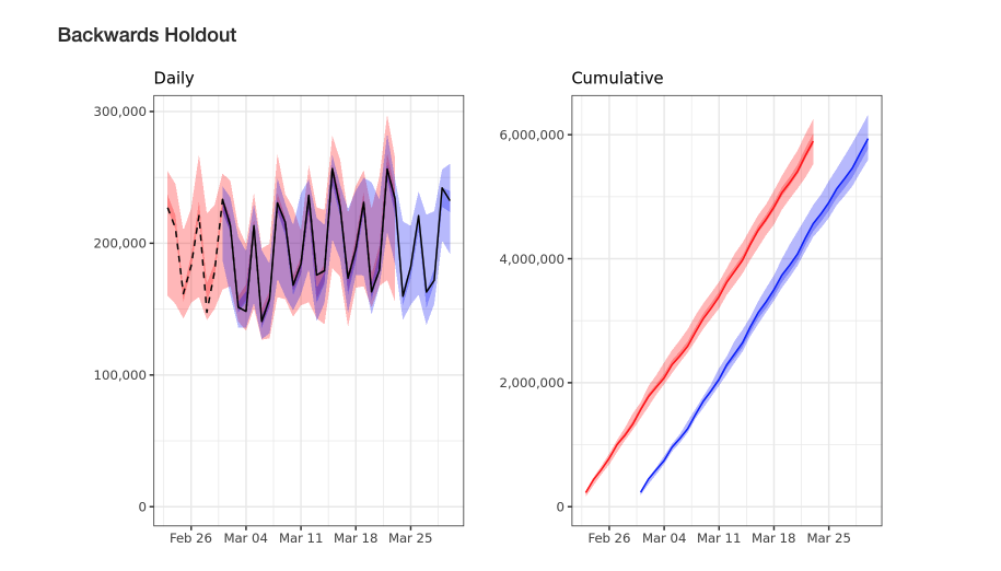
A model run automatically produces a 30 day holdout for the last 30 days in your model. The plots above compares the previous daily and cumulative holdout with the new model's holdouts. Poor holdout performance may indicate missing spikes, missing marketing spend, or a poorly specified model.

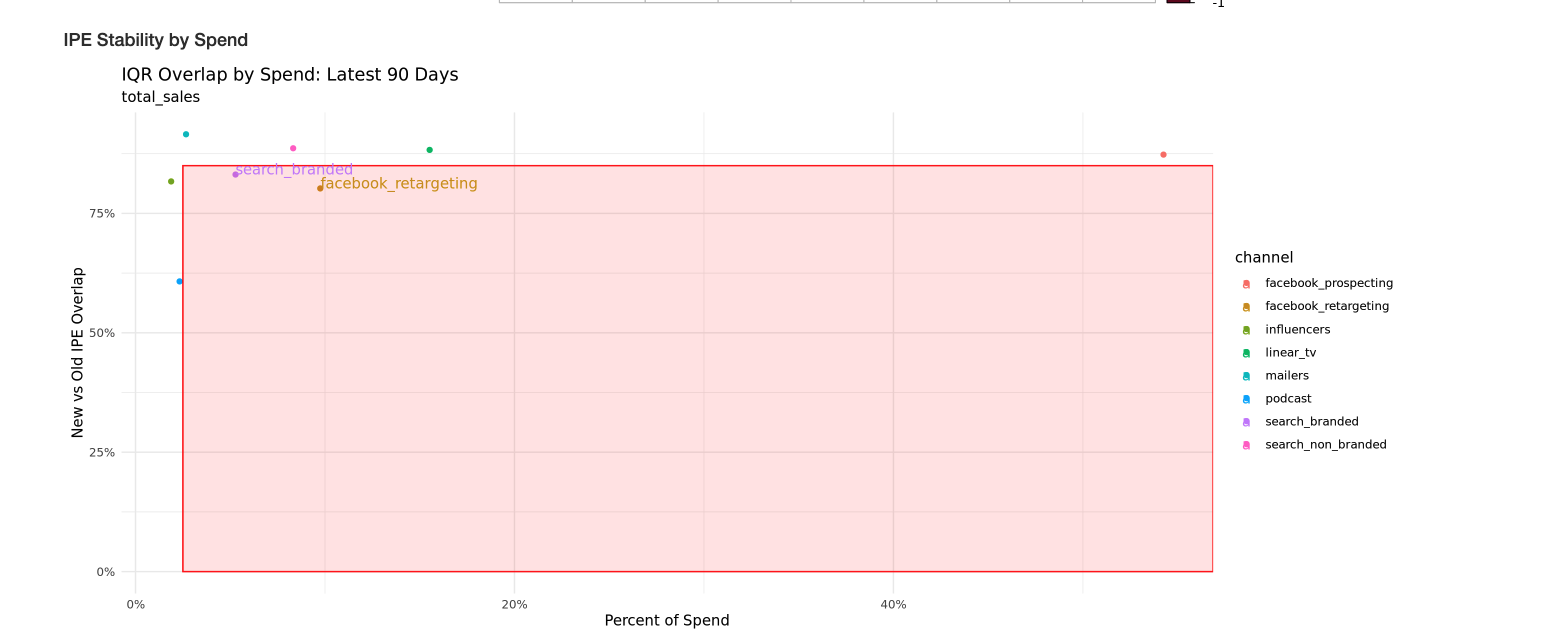
This plot emphasizes the channels showing the most instability. Large channels with little overlap in their confidence intervals compared to the last run are a cause for concern and should be investigated. Those channels will be labeled in the red box.

This text block indicates what channels had historical changes in spend and what priors changed between runs. Changing priors between runs can make the model unstable. Changes to the historical spend can cause priors to change, which will show up here.

Note: Saturation priors are currently reported on model scale instead of world scale. Because the model scale can change week to week (depending on fluctuations in the data), we expect small fluctuations in the model scale saturation priors. Other priors are reported on the world scale and ideally stay stable week to week.

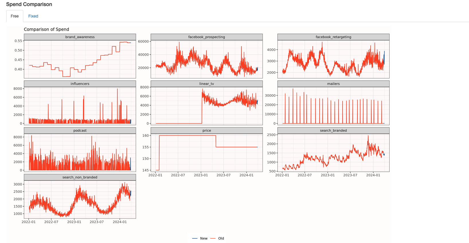
The next chart shows the reported spend and context variables for both the old and new run. This can be helpful to see changes in what was previously modeled vs. what is being modeled now.

The full comparison chart compares changes in model inferences. In period effect summarizes how much credit marketing activities are getting for sales, the intercept shows our estimate of organic, and spikes shows what we're attributing to spike variables.

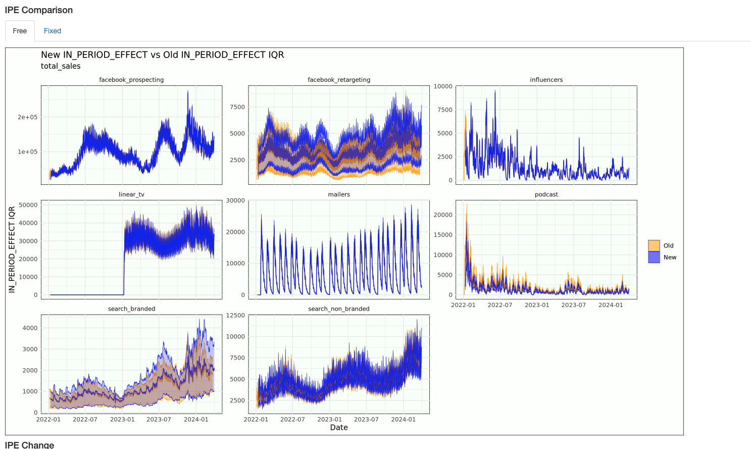
The above two graphs show how our channel inferences changed between runs. The top graph shows the "in period effect" or how much of the dependent variable we attribute to that channel each day. The bottom graph shows the estimated ROI for that channel across time.

Parameter Recovery Dashboard

The parameter recovery dashboard helps us know how well we're estimating the true parameters when the true parameters are known. Most graphs will compare three things:

The prior (quantiles of all draws from the prior only run)
The posterior (the quantiles of all draws from the run with the simulated depvar)
The truth (the value of the parameter that was used to produce the simulated depvar)

At the top we report CRPS statistics. The CRPS can be thought of as a Bayesian version of MAPE that takes into account the uncertainty distribution in addition to the point estimate (if two predictions have the same point estimate, the one with less uncertainty will have lower CRPS). The CRPS ratios reported here are the ratio of the CRPS scores on the ROI recovery from the posterior divided by the CRPS scores from the prior. Scores above one mean your posterior had more error than the prior, while lower scores indicate better parameter recovery. We primarily look at the spend weighted ratio, as that gives more weight to the channels with the most spend.

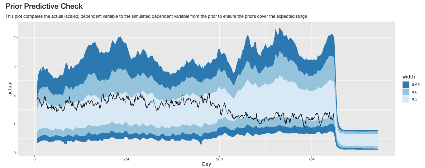
The prior predictive graph plots the actual dependent variable inside the simulated range of possible dependent variables from the prior. If the actual dependent variable is outside the prior, we're putting small prior weight on the real outcome, so we probably have an error in how we're setting our priors.

Graphs comparing the prior, simulated dependent variable run, and truth are available for all of the following parameters of interest:

Intercept
ROIs
Time Shifts
Spend response curves
Saturation parameter
Lower funnel betas/intercept
Context variable effects

Stability Loop Outputs

The stability loop run type will produce a run analysis dashboard for each consecutive pairing of model runs, so if you do use the setting n_periods = 3, you will get three stability loop dashboards. Additionally, you will get a "unified stability loop dashboard" which takes the most salient information from the individual dashboards and combines it on a single dashboard. This is helpful in comparing across dashboards.

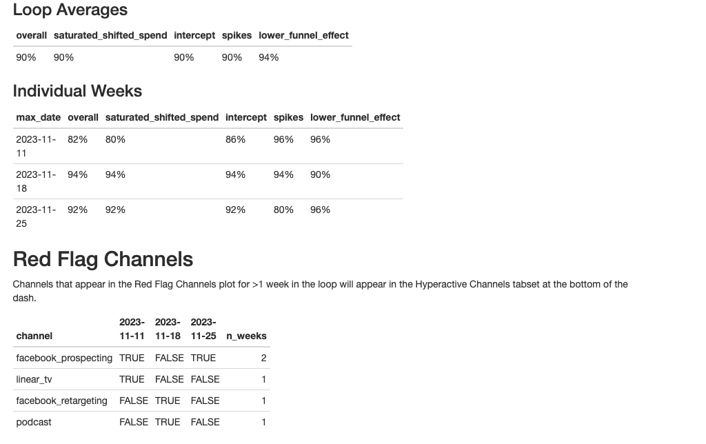
At the top of the unified dashboard, you get average stability metrics across all runs, metrics by run, and a table showing how many times each channel was "red-flagged" as particularly unstable. All graphs underneath this are equivalent to graphs in the run analysis dashboard and can be used to quickly determine what parts of the model most need attention.

Holdout Dashboard

A single holdout dashboard will be created summarizing all the holdout models you ran. The holdout analysis involves creating an out of sample forecast by taking the spend in the forecast period and predicting the dependent variable. We then compare the forecast with the truth to determine if the model is accurately modeling future time periods.

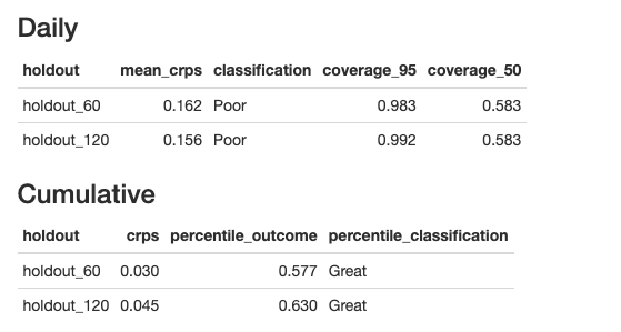
The statistics at the top quantify the quality of the holdouts. A cumulative result in the 25th-75th percentile of the forecast is considered great, while a result within the 2.5-97.5 percentile is considered good. CRPS scores can be especially useful when comparing across models, as a lower holdout CRPS generally indicates a better model.

The daily graph shows the actual KPI with our confidence interval (IQR in darker color, 95% in lighter). This can be useful in assessing fit on individual days, particularly around big spikes.

The cumulative forecast shows the cumulative sum of the dependent variables and our predictions.